
Monte Carlo Trading: Master Risk Simulation in 2026
- Discipline AI

- 4 days ago
- 10 min read

What is Monte Carlo simulation in trading?
Monte Carlo trading simulation takes your historical trade results and reshuffles them into thousands of random sequences. Each sequence produces a different equity curve. Run enough of them and you get a distribution of outcomes, not a single path, which is exactly what risk management requires.
The core insight is deceptively simple: your backtest shows one ordering of trades. That ordering might have been lucky or unlucky. You have no way to know which without testing other orderings. Monte Carlo simulation does exactly this, exposing the range of luck-driven outcomes hiding inside any single backtest result.
Key features of a Monte Carlo analysis for traders:
Synthetic equity curves: Thousands of alternate account paths built from the same trade set
Drawdown distributions: Not just the backtest’s max drawdown, but the realistic range across all simulations
Probability of Profit: The share of simulated runs that finish above the starting balance
Probability of Ruin: The share of runs that breach a critical drawdown threshold
Luck vs. skill assessment: Whether the original backtest is an outlier among simulated paths or a representative result
How Monte Carlo simulation works on your trading strategies
The mechanics are straightforward, even if the math underneath is not.
Step 1: Extract trade results. Pull the P&L of every individual trade from your backtest, each one as a discrete outcome with its dollar or percentage value.

Step 2: Reshuffle or resample. Either permute the trades (randomize order without replacement, so every trade appears exactly once) or bootstrap them (draw with replacement, so some trades repeat and others get skipped). Permutation isolates sequence risk; bootstrap introduces variation in final equity as well.
Step 3: Simulate the equity curve. Apply the reshuffled sequence to the starting balance using fixed fractional sizing. Because position size is a percentage of the current balance, results compound: dollar risk shrinks during drawdowns and grows during run-ups.
Step 4: Repeat. Run several thousand iterations for statistically stable output. Below this count, percentile estimates wobble run to run. Beyond it, the marginal improvement in precision is negligible for most trading applications.
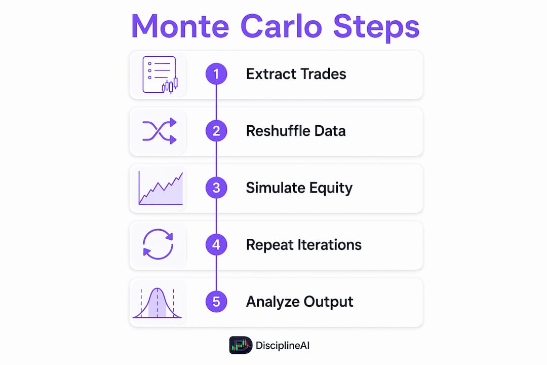
The output is a distribution of equity curves, drawdowns, and final balances. That distribution is what you actually need to make sizing decisions.
Interpreting key metrics from Monte Carlo trading simulations
The raw output of a Monte Carlo run is a fan of equity curves. Reading it correctly is where most traders either gain real insight or get lost.
Confidence bands plot three curves from the simulation distribution:
5th percentile: Near worst-case. Only 5% of simulations performed worse.
50th percentile (median): The middle outcome. Half did better, half did worse.
95th percentile: Near best-case. Only 5% of simulations performed better.
If the 5th percentile curve still ends in profit over your planned trading horizon, the strategy’s edge survives bad sequencing. If it goes negative, the strategy may be profitable on average but carries real loss risk over any single evaluation period.
Drawdown distributions answer the question single-path backtesting cannot. If your backtest showed a maximum drawdown but the 95th percentile Monte Carlo drawdown is substantially higher, your strategy is roughly twice as risky as the backtest suggests. That 28% figure is the one to use when setting position sizes and ruin thresholds.
Metric | What it tells you | How to use it |
Probability of Profit | % of simulations finishing above starting balance | Gauge overall edge strength |
Probability of Ruin | % of simulations breaching critical drawdown | Hard limit for position sizing |
Median max drawdown | Typical worst drawdown across simulations | Set baseline capital expectations |
P95 max drawdown | Near worst-case drawdown | Primary sizing and ruin threshold input |
Confidence band width | Gap between 5th and 95th percentile curves | Measure of sequence sensitivity |
Probability of Profit and Probability of Ruin are the two numbers that most directly translate simulation output into a go/no-go decision on live capital.
Why traders use Monte Carlo simulations and when it matters most
A single backtest is one data point. Monte Carlo turns it into a distribution. That shift from point estimate to range is the entire value proposition.

Detecting overfitting. Monte Carlo reveals overfitting by showing whether the original backtest is an outlier among simulated paths. If the backtest’s equity curve sits near the 95th percentile of all simulations, the historical result depended heavily on favorable sequencing, not repeatable edge. Identical win rate and risk-reward can produce drastically different equity curves depending on trade order alone.
Stress testing before live deployment. Traders use Monte Carlo to simulate trade skipping and sequencing errors, the kind of real-world friction that clean backtests ignore. A strategy that looks solid on paper can show 85% drawdown potential when just 12% of trades are missed.
Prop firm challenge preparation. Prop firm challenges introduce hard constraints: hit a profit target before breaching a drawdown limit within a fixed number of days. Monte Carlo outputs a pass rate across thousands of simulated challenges, letting you calculate how many attempts a strategy should require on average before passing.
Periodic reassessment with live data. Running the simulation on live trade results, once enough trades have accumulated, updates risk assumptions to reflect actual execution rather than idealized backtest conditions. Live results typically show wider drawdowns and lower win rates than backtests due to slippage and market changes.
Pro Tip: Run Monte Carlo before you risk a single dollar live. The simulation costs nothing. The information it reveals about your strategy’s true drawdown range is worth more than any single trade.
How to apply Monte Carlo results to real trading decisions
The output is only useful if it changes how you size and manage positions. Here is how to translate simulation results into concrete adjustments.
Focus on the 5th percentile, not the median. Plan around near worst-case sequencing. The median outcome is what an average run looks like; the 5th percentile is what a bad-luck run looks like. Sizing for the median means you are underprepared for the runs that actually test your discipline.
Size based on the P95 drawdown. Take the 95th percentile drawdown from the simulation and scale position sizes so that drawdown stays within your actual tolerance. If P95 drawdown exceeds your maximum tolerance, scale positions down to keep drawdown within your limit. That math is straightforward and directly protects your capital.
Validate ruin probability at your chosen size. After scaling, confirm that the Probability of Ruin at the new size falls below an acceptable threshold. For most serious traders, anything above 1% ruin probability at a given sizing is a signal to reduce further. This connects naturally to risk management principles that treat capital preservation as the primary constraint.
Do not use Monte Carlo for optimization. Running simulations to find parameter sets that produce better-looking outputs is a form of meta-overfitting. Experts recommend validating robustness across many randomized sequences instead of chasing cleaner percentile curves. The goal is to understand variance, not to engineer it away.
Update inputs with live trade data. Once live trading has produced enough trades for meaningful statistics, rerun the simulation using actual results. Updating Monte Carlo inputs with live data ensures sizing reflects real performance, not idealized backtest assumptions. This mirrors how AI-driven financial tools continuously recalibrate models as new data arrives.
Advanced insights from practitioners using Monte Carlo simulation
The standard reshuffle simulation makes one assumption that often fails in real markets: trade independence. Losses cluster. Momentum persists. Mean reversion creates serial correlation in returns. When that structure exists, plain reshuffling produces confidence intervals that are too tight.
Block bootstrap addresses this by reshuffling contiguous blocks of trades rather than individual ones. This preserves local autocorrelation while still randomizing the global sequence. For trend-following strategies or carry trades where multi-day persistence is common, block bootstrap gives more realistic drawdown estimates than standard permutation. The block length should roughly match the autocorrelation horizon of the return series.
Monte Carlo complements out-of-sample testing but does not replace it. Walk-forward analysis confirms that strategy parameters work on unseen data across multiple time windows. Monte Carlo confirms that the validated edge survives bad sequencing. Use walk-forward first to establish that the edge is real, then Monte Carlo to understand how to size for it. Neither test alone is sufficient.
Randomized position sizing within simulations models execution constraints more realistically. Advanced simulation methods include varying position size within each run to prevent the unrealistic assumption of perfect, consistent execution on every trade.
Sample size matters. A simulation built on 20 trades produces wide, unreliable confidence intervals. The distribution stabilizes as the trade count grows. Practitioners generally treat results from fewer than 30 trades as directional at best, and wait for a larger sample before making hard sizing decisions based on Monte Carlo output.
Pro Tip: A Monte Carlo output that looks too clean is a warning sign, not a green light. Real strategies with genuine edge still show wide confidence bands. If your fan chart is suspiciously narrow, check whether your trade sample is large enough or whether the simulation assumptions match your actual trading conditions.
Step-by-step Monte Carlo implementation with Python
The fastest way to build intuition for Monte Carlo is to run it yourself. Here is a working Python workflow covering the two most useful methods.
Method 1: Reshuffle (sequence risk)
import numpy as np

def reshuffle_monte_carlo(trades, n_simulations=1000):
    n_trades = len(trades)
    max_drawdowns = np.zeros(n_simulations)

    for i in range(n_simulations):
        shuffled = np.random.permutation(trades)
        equity = np.cumsum(shuffled)
        running_max = np.maximum.accumulate(equity)
        drawdown = running_max - equity
        max_drawdowns[i] = drawdown.max()

    return max_drawdowns

trades = np.array([200, -150, 300, -100, 250, -200, 180, -90])
drawdowns = reshuffle_monte_carlo(trades, n_simulations=5000)
print(f"P50 drawdown: {np.percentile(drawdowns, 50):.2f}")
print(f"P95 drawdown: {np.percentile(drawdowns, 95):.2f}")
The key output is the drawdown distribution. If your backtest showed a $2,000 max drawdown but the 95th percentile from Monte Carlo is substantially higher, fund your account to cover that level of risk.
Method 2: Drawdown confidence intervals
def drawdown_confidence(trades, n_simulations=1000,
                        confidence_levels=[0.50, 0.90, 0.95]):
    drawdowns = reshuffle_monte_carlo(trades, n_simulations)
    return {level: np.percentile(drawdowns, level * 100)
            for level in confidence_levels}

results = drawdown_confidence(trades)
for level, dd in results.items():
    print(f"{int(level*100)}th percentile drawdown: {dd:.2f}")
For traders without a Python environment, free browser-based tools accept MT4, MT5, and cTrader backtest reports and run up to 5,000 permutations instantly, with drawdown confidence intervals at the 50th, 90th, 95th, and 99th percentiles.
How Monte Carlo compares to other risk management methods
Monte Carlo is one tool in a larger validation process. Each method catches different failure modes.
Standard backtesting produces a single equity path on historical data. It tells you what happened under one specific sequence. It cannot tell you whether that sequence was representative or lucky. Monte Carlo fills exactly this gap.
Out-of-sample testing and walk-forward analysis test whether strategy parameters generalize to unseen data. This catches overfitting to specific historical noise. Monte Carlo does not test this. A strategy can pass Monte Carlo and still be overfit to the historical period it was built on. The two methods are complementary, not interchangeable.
Stress testing applies extreme but plausible market scenarios (a flash crash, a liquidity gap, a correlation breakdown) to evaluate strategy behavior under tail conditions. Monte Carlo reshuffles known trade outcomes; stress testing asks what happens when conditions fall outside the historical sample entirely.
Risk of ruin formulas give a single closed-form probability based on average edge and fixed position size. Monte Carlo uses the actual trade distribution, including variable win and loss sizes, and produces a full range of outcomes. Risk of ruin is faster for quick sizing checks; Monte Carlo is more granular for thorough validation. Use both: risk of ruin for a rapid sanity check, Monte Carlo for the full picture before committing live capital.
The practical workflow is: walk-forward analysis first to confirm the edge is real, then Monte Carlo to understand how to size for it, then risk of ruin to set the final position size.
Best practices for selecting inputs and distributions
Garbage in, garbage out applies more directly to Monte Carlo than to almost any other analysis. The simulation is only as reliable as the inputs you feed it.
Use measured win rates, not aspirational ones. With a small sample, your true win rate could easily be 5–10 percentage points below what you have observed. Re-run the simulation with a pessimistic win rate to see how the picture changes before committing to a position size.
Match the simulation method to your strategy type. Permutation (reshuffle without replacement) isolates sequence risk and is appropriate for most strategies. Bootstrap (resample with replacement) introduces variation in final equity and is better for estimating uncertainty around backtest results. For autocorrelated return series, block bootstrap is the right choice.
Set the iteration count at 5,000–10,000. A minimum of 1,000 produces usable results. For more statistically stable output, 5,000 to 10,000 iterations is standard. Beyond 10,000, the marginal improvement in precision is negligible for most trading applications.
Include realistic execution assumptions. Standard Monte Carlo models assume trade independence, fixed win rate, and no fees or slippage. Real markets violate all three. Monte Carlo often underestimates drawdowns because it ignores liquidity constraints and assumes losses do not cluster. Treat the output as a variance map, not a forecast, and add a buffer to the P95 drawdown before setting your final position size.
Recalibrate when market conditions shift. A simulation built on bull-market trades will underestimate drawdowns in a mean-reverting or high-volatility regime. Watching for signs of overtrading or parameter drift in live results is one signal that a recalibration is due.
Use the 5th percentile as your planning number, not the median. The lower quantile is your honest planning figure. A Sharpe ratio with a wide confidence interval is a fundamentally different decision than the same point estimate with a tight one. For max drawdown, the 95th percentile bootstrap value is the right capital-planning number, not the single observed max drawdown in your backtest sample.
Key Takeaways
Monte Carlo simulation transforms a single backtest path into a distribution of outcomes, making the P95 drawdown the only defensible basis for position sizing.
Point | Details |
Reshuffle reveals sequence risk | Randomizing trade order shows the realistic drawdown range your backtest cannot capture alone. |
Size for the P95 drawdown | Use the 95th percentile simulated drawdown, not the backtest figure, to set position sizes. |
5,000–10,000 iterations for stable output | Fewer than 1,000 runs produce unreliable percentile estimates; beyond 10,000 adds little precision. |
Monte Carlo does not replace out-of-sample testing | Walk-forward analysis confirms edge is real; Monte Carlo shows how to size for it. |
Update inputs with live trade data | Recalibrate the simulation once live results accumulate to keep risk sizing accurate. |
Take your risk analysis further with Disciplineaiapp

Monte Carlo simulation tells you the range of outcomes your strategy can produce. Acting on those insights requires the right tools around you. Disciplineaiapp combines AI-generated trade setups, confidence scoring, position sizing calculators, and detailed performance analytics in one platform built for active traders. The behavioral coaching and stand-aside protection features help you stay disciplined through the exact drawdown sequences Monte Carlo warns you about.
Explore what Disciplineaiapp’s trading intelligence features can add to your risk management process, or visit the AI Learning Center for deeper strategy analysis resources.
Recommended

Comments